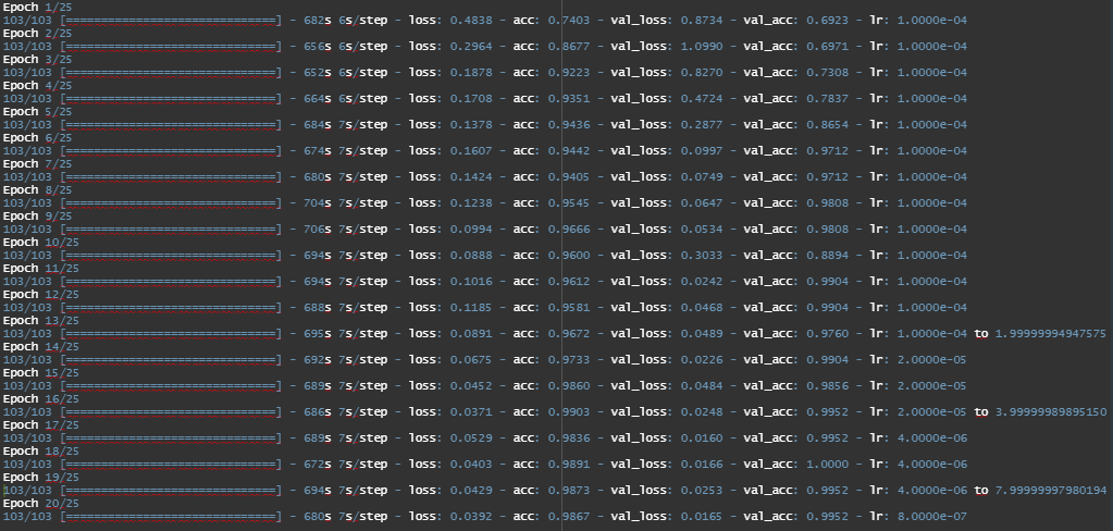
Spoiler Alert ! One of the networks achieve a98 % classification accuracy.
A Binary Unbalance Classification Example
Breast Cancer is the commonest malignancy among women globally. It has now surpassed lung cancer as the leading cause of global cancer incidence in 2020, with an estimated 2.3 million new cases, representing 11.7% of all cancer cases. In India, the incidence has increased significantly. As per Globocan data 2020, in India, breast cancer accounted for 13.5% of all cancer cases and 10.6% of all deaths.
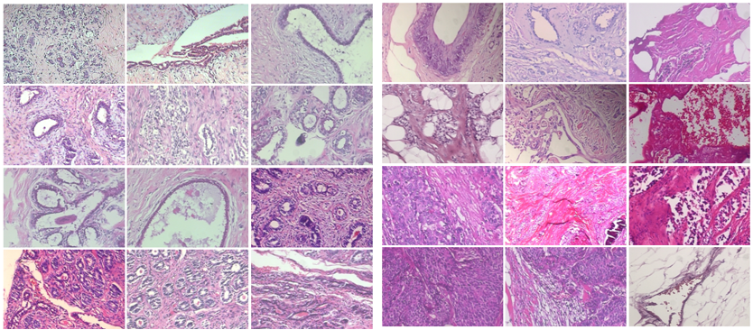
Glimpse into our Data
X-ray : Benign -&- Malignant
Seeing these images side by side, one cannot make out which is cancerous and which is benign.
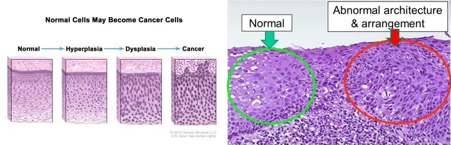
Evolution of Cancer
This sort of gives us an indication how cancer cells look different from normal ones.
The dataset used can be access from the Laboratório Visão Robótica e Imagemwebiste. The dataset is divided into two main groups: benign & malignant tumors. Malignant tumour is a synonym for cancer: lesion can invade and destroy adjacent structures (locally invasive) and spread to distant sites (metastasise) to cause death. We use the 100x Magnification images here.
Data Preparation
Train Validation Test Split
We will split the data into 3 parts for training, validating and testing the model’s performance. We use about 1600 images for training and 200 for testing and validating.
Original Data
Total
Train
Validation
Test
Benign
640
512
64
64
Malignant
1424
1136
144
144
Total
2064
1648
208
208
Based on the above split, we can use batch_size = 16. Batch size is one of the most important hyper-parameters to tune in deep learning. If the value is low, the network will end up training poorly. If high, then the network does not generalise well. Thus, the steps_per_epoch = 103 for train, 13 for validation and test. (Because 16*103 = 2064 and 13*15 = 208).
The 1st chunk of code deals with setting-up respective directories. Then we transfer images from the Malignant and Benign folders to Train-Validation-Test folders. To randomly select files, we use sample() to create indexes.
Code
# Set Directorybase_dir ="C:/Users/KUNAL/Downloads/#R coding/#Books/covered/#Book - Manning - Deep Learning with R and Keras/## Article/100x"benign_dir =file.path(base_dir, "benign")malignant_dir =file.path(base_dir, "malignant")# Create respective folderstrain_dir =file.path(base_dir, "train")validation_dir =file.path(base_dir, "validation")test_dir =file.path(base_dir, "test")# dir.create(train_dir); dir.create(validation_dir); dir.create(test_dir)# Creating respective sub-folderstrain_benign_dir <-file.path(train_dir, "benign")validation_benign_dir <-file.path(validation_dir, "benign")test_benign_dir <-file.path(test_dir, "benign")train_malignant_dir <-file.path(train_dir, "malignant")validation_malignant_dir <-file.path(validation_dir, "malignant")test_malignant_dir <-file.path(test_dir, "malignant")# dir.create(train_benign_dir); dir.create(validation_benign_dir); # dir.create(test_benign_dir) ; dir.create(train_malignant_dir); # dir.create(validation_malignant_dir); dir.create(test_malignant_dir)# Reading in the file namesbenign_fnames =paste0("benign (", 1:640, ").png")benign_fnames =sample(benign_fnames) # randomize picturesmalignant_fnames =paste0("malignant (", 1:1424, ").png")malignant_fnames =sample(malignant_fnames)# creating indices for train-validation-test splitbenign_index =c(rep(1,512),rep(2,64),rep(3,64))benign_index =sample(benign_index) # randomize indexesmalignant_index =c(rep(1,1136),rep(2,144),rep(3,144))malignant_index =sample(malignant_index)# separating file names as per indicestrain_benign_fnames = benign_fnames[benign_index==1]validation_benign_fnames = benign_fnames[benign_index==2]test_benign_fnames = benign_fnames[benign_index==3]#train_malignant_fnames = malignant_fnames[malignant_index==1]validation_malignant_fnames = malignant_fnames[malignant_index==2]test_malignant_fnames = malignant_fnames[malignant_index==3]# copying files to respective folders# file.copy(file.path(<old_location>, <file_name>),file.path(<new_location>))file.copy(file.path(benign_dir, train_benign_fnames),file.path(train_benign_dir))file.copy(file.path(benign_dir, validation_benign_fnames),file.path(validation_benign_dir))file.copy(file.path(benign_dir, test_benign_fnames),file.path(test_benign_dir))file.copy(file.path(malignant_dir, train_malignant_fnames),file.path(train_malignant_dir))file.copy(file.path(malignant_dir, validation_malignant_fnames),file.path(validation_malignant_dir))file.copy(file.path(malignant_dir, test_malignant_fnames),file.path(test_malignant_dir))# Checkingcat("total training benign images:", length(list.files(train_benign_dir)), "\n")cat("total training malignant images:", length(list.files(train_malignant_dir)), "\n")cat("total validation benign images:", length(list.files(validation_benign_dir)), "\n")cat("total validation malignant images:", length(list.files(validation_malignant_dir)), "\n")cat("total test benign images:", length(list.files(test_benign_dir)), "\n")cat("total test malignant images:", length(list.files(test_malignant_dir)), "\n")
The count of images for train-validate-test matches the division we saw above. Clearly, this is UnbalancedClassification Problem. So we must assign weights to the classes :
For Benign : 2064/(2*640) = 1.6125
For Malignant : 2064/(2*1424) = 0.72471910112
Convolution Neural Network
The next chunk of codes involve setting up and training a basic convolution neural network.
A Callback is a list of control-instructions which the model looks during the training process. It helps interrupts training and make changes accordingly. Some of the callbacks we’ll use :
callback_early_stopping() -> This interrupts training once a target metric being monitored has stopped improving for a fixed number of epochs and helps avoid overfitting. This is done if there is no improvement in validation loss/error after ‘patience = 3’ number of epochs.
callback_model_checkpoint() -> This allows us to continually save model during training - save version of model with best performance.
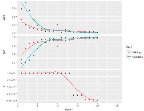
callback_reduce_lr_on_plateau() -> This allows the learning rate to fall if there is no improvement in the validation loss/error. The learning rate is reduced by a factor of 0.3 after there is no improvement in ‘patience = 3’ number of epochs.
Table 1 : How different CNN model structures perform
Sl.
Model Structure
Epochs
Training
Validation
Test
Optimizer :
Adam
1
5 Conv layers with (32,32,64,64,128) & 2 dense layers with (128,64) hidden units
12/25
82.58%
85.10%
81.25%
2
5 Conv layers with (32,32,64,64,128) & 2 dense layers with (64,32) hidden units
23/25
87.08%
87.98%
82.69%
3
5 Conv Layers with (32,32,64,128,128) & 2 dense layers with (128,64) hidden units
11/25
87.08%
87.98%
82.69%
Optimizer :
RMSprop
4
5 Conv Layers with (32,32,64,64,128) & 1 dense layer with 512 hidden units
14/25
85.92%
87.98%
84.13%
5
5 Conv Layers with (32,32,64,64,128) & 2 dense layers with (64,32) hidden units
11/25
87.56%
88.46%
87.01%**
The 5th Model in above table is so far the best performing model with a Test Accuracy of 87%.
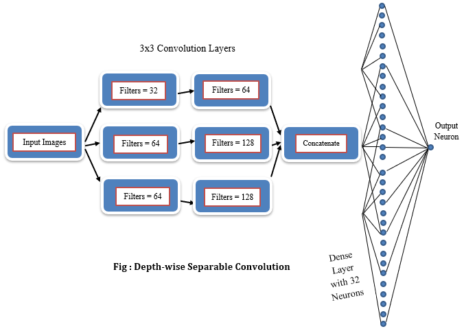
Depth-wise Separable Convolution
The idea is to learn spatial features from each channel of its input, independently, before mixing output channels via a point-wise convolution (1x1 convolution). It requires significantly fewer parameters and involves fewer calculations thus, the training process is faster. It tends to learn better representations using less data, resulting in better-performing models. It is especially helpful when dealing with small datasets.
Table 2 : How different Separable CNN model structures perform
Sl.
Model Structure
epochs
Training
Validation
Test
1
(32,64) (32,64) (64,128) (32)
8/25
69.93%
69.23%
69.23%
2
(32,64) (64,128) (128,256) (32)
4/25
57.77%
30.77%
30.76%
3
(64,128) (64,128) (64,128) (32)
5/25
68.23%
69.23%
69.23%
4
(64,128) (64,128) (128,256) (32)
4/25
34.34%
30.77%
30.76%
5
(32,64) (64,128) (64,128) (64)
10/25
77.91%
82.21%
77.40%
6
(16,32) (32,64) (64,128) (32)
11/25
83.19%
87.02%
79.80%
7
(32,64) (64,128) (64,128) (32)**
20/25
85.44%
87.98%
85.58%
The 7th Model from the above table is the best performing among all the Depth-wise Separable CNNs trained here. It has 2 layers with 32 and 64 hidden units in the first separable layer. 64,128 in second and third separable layers respectively. It ends up with a dense layer with 32 hidden units.
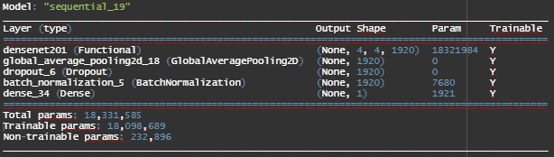
DenseNet201
DenseNet-201 is a convolution neural network that is 201 layers deep. The network was trained on more than a million images from the ImageNet database. This pre-trained network can classify images into 1000 object categories such as keyboard, mouse, pencil, and many animals. As a result the network has learnt rich feature representations for a wide range of images which will be helpful for our Cancer X-ray image classification problem.